

In today's fast-paced business landscape, staying ahead of the competition requires efficient and effective solutions. According to Microsoft’s Work Trend Index, nearly 70% of employee report that they don’t have sufficient time in the day to focus on “work”, with more time being spent Communicating than Creating.
Microsoft 365 Copilot is designed, with Microsoft’s cloud trust platform at its core, to allow for employees to both be more productive, reduce the time spent searching for information, performing mundane tasks, and other low-value activities.
Power BI
Power BI connects to 115+ data sources. A webpage connector is very useful and enables data stored on websites to be mashed up and analyzed. When several webpages in a given URL share the same structure and content (e.g., a page for each year or category), the creation of a parameter for the URL and a function to replicate the Power Query code can import all of the data into a single data-set. This blog post will demonstrate how to do just that.
Introduction
The data we are interested in is NFL game data over several years. This data is maintained at Pro Football Reference https://www.pro-football-reference.com. Seasons are stored on separate pages as shown in the following table:
|
2019 |
https://www.pro-football-reference.com/years/2019/games.html |
|
2018 |
https://www.pro-football-reference.com/years/2018/games.html |
|
2017 |
https://www.pro-football-reference.com/years/2017/games.html |
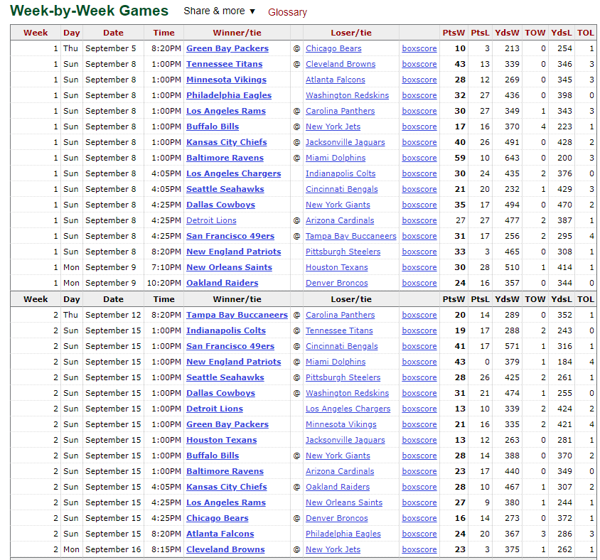
On each page, we are interested in the data available in the “Week-by-Week Games” table.
Build the Data Transformation
Here are the steps to retrieve, transform, and analyze the data for the past 10 seasons. We will create the transformation steps for one season then convert that script into a function that can be repeated over any number of pages (years) of data on the website.
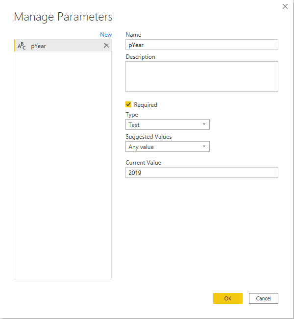
Open Power BI desktop and click “Transform Data” in the Home Ribbon. This opens Power Query Editor, where we will define our data transformation. Create a parameter, pYear, to store the year/season from which we wish to retrieve data. Click on “Manage Parameters” and click “New.” We will store this as a text type since we will be plugging this into a URL.
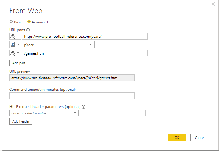
Now, click “New Source,” and select “Web” and “Advanced” as shown below. We are breaking the URL into 3 pieces, a first part (text), the year (parameter pYear), and the page name (text).
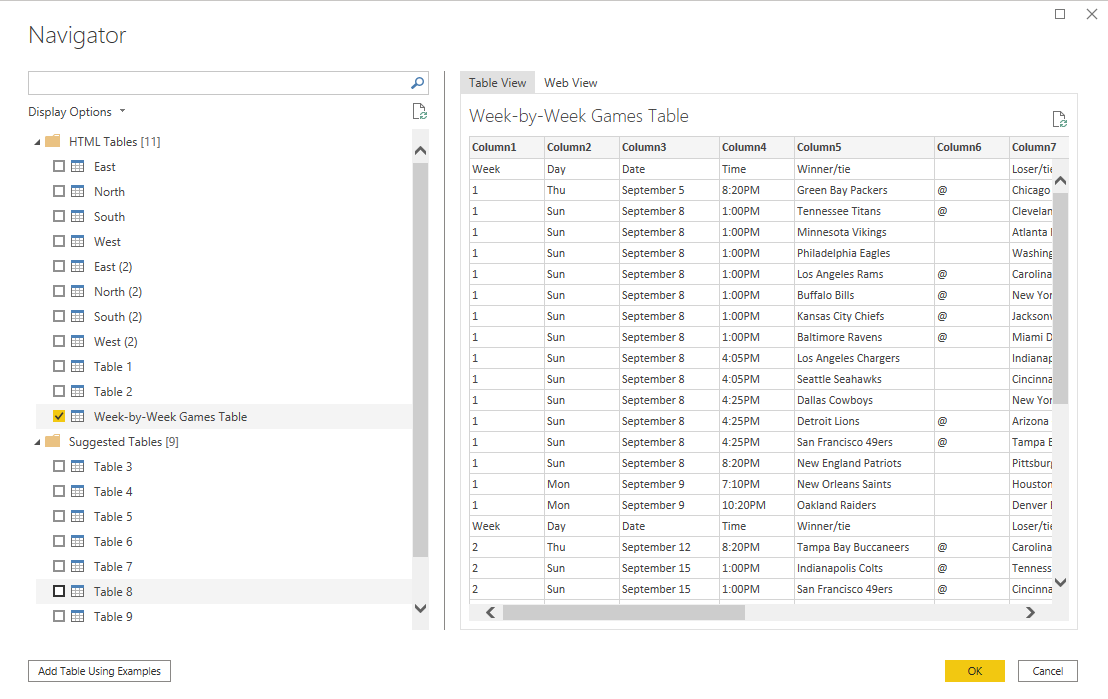
Click OK to preview the data and check the “Week-by-Week Games Table” to preview the data.
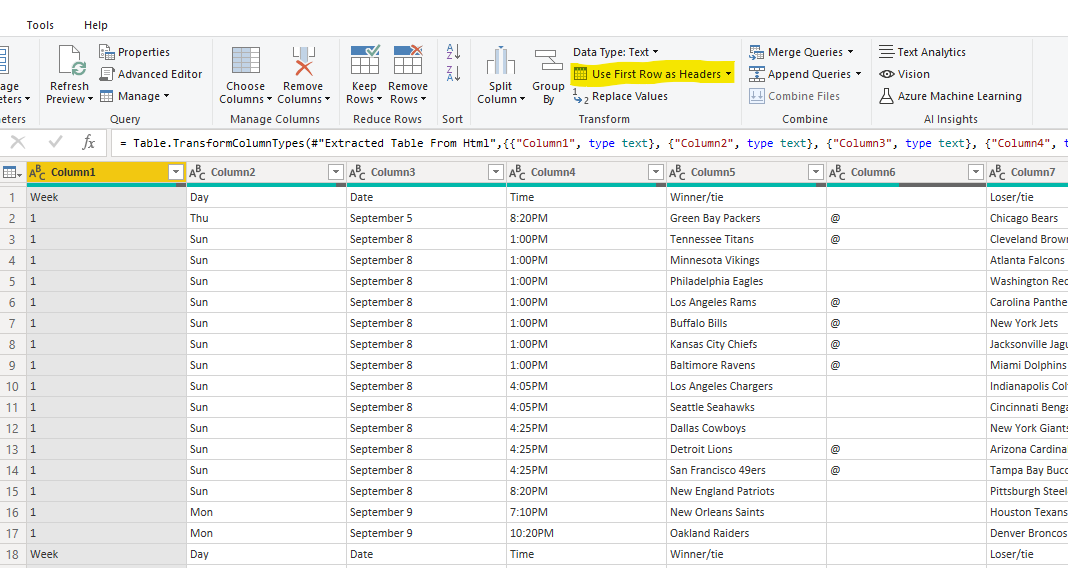
Click OK to import the data. At this point, we will need to do some data transformations before we can analyze it. One of the first transformations to perform is to promote the first row as headers. Click on “Use First Row as Headers” in the Home ribbon of Power Query Editor.
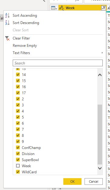
The first column, “Week” stores the season week number and playoffs round (e.g., WildCard, Division, ConfChamp). It also has the repeating header, “Week” and there are some blank values. To remove the blanks, click the arrow in the header, and select “Remove Empty.” Similarly, uncheck the box next to “Week” and click OK.
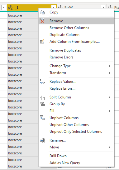
One of the columns holds links to the boxscore for each game. This is not necessary for our dataset, so let’s remove it by right-clicking on the column header and selecting “Remove.”
The table stores the winning team and the losing team in dedicated columns, with a column containing the “@” symbol to denote if the game was played in the losing team’s stadium. This column does not have a name, so rename it to “Location” (double-click the header and type “Location”).
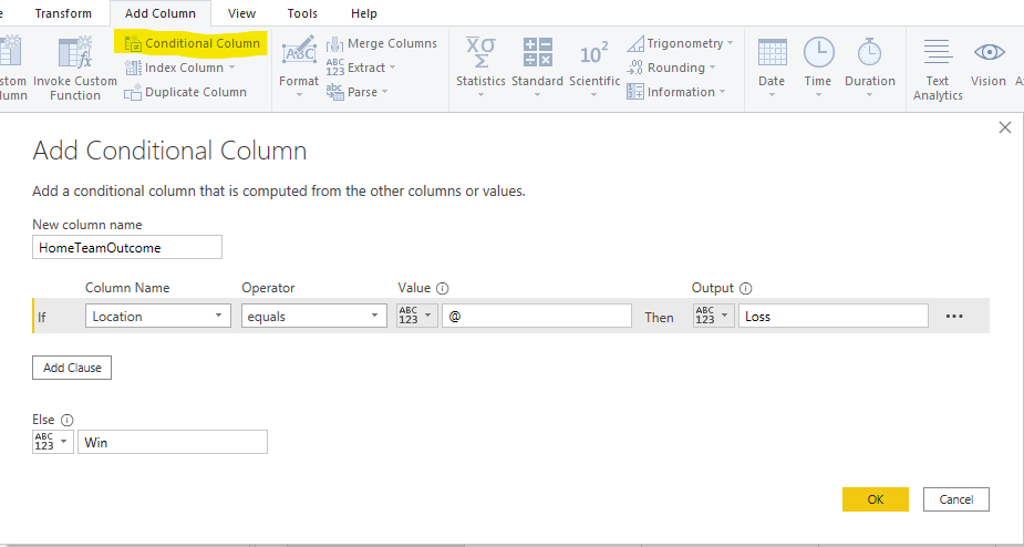
There is some other interesting information we can get from this dataset, like how often the home team loses. To do this, click “Add Column” and “Conditional Column.” We will name this “HomeTeamOutcome,” and the logic will be that if the “Location” column equals “@” then the home team lost. See below.
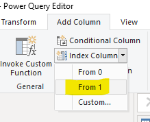
Another useful column to have is an index column with a unique value for each row. This way, the model can contain measures that count the number of distinct values of an ID field, as an example. We will call this “GameID” and create it by clicking “Index Column” in the “Add Column Ribbon.” We want our first value to be 1, not zero, so we select “From 1” in the drop-down. To rename the resulting column named “Index,” double-click the column header and type “GameID.”
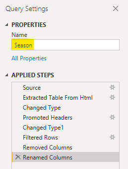
There is a lot more we could do to model this data, but for the purposes of the demonstration, we will go ahead and convert this to a function and retrieve data for the last 10 seasons. We should rename the table to “Season” by editing the Name in the Query Settings box.
Create the fnGetSeason Data Retrieval Function
To convert this into a function, right-click on the Season query in the Queries pane and select “Create Function.”
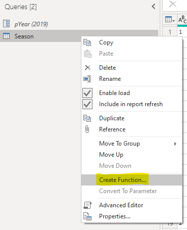
Power BI detects that a parameter (pYear) is used in the function, and we can name the function “fnGetSeason.”
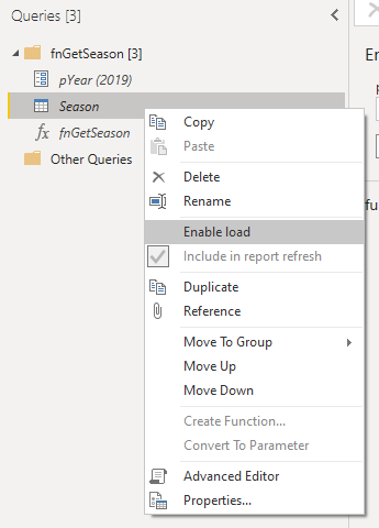
Click OK and the function is created. Since we do not want the “Season” query to load in the report, right-click and uncheck “Enable Load” in the dialog box.
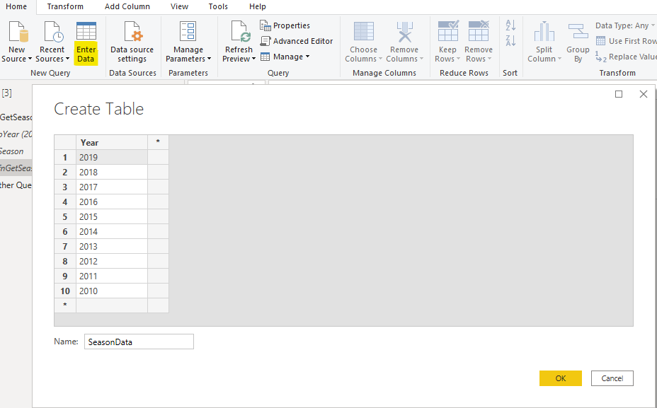
We will need values to input into the function, so we will create a table with 10 rows, one for each of the last 10 seasons. On the Home ribbon, click “Enter Data” and populate it as follows. Double click on the column header to name the column “Year” and name the table “SeasonData.” Click OK and there is now a table from which we will use our fnGetSeason function.
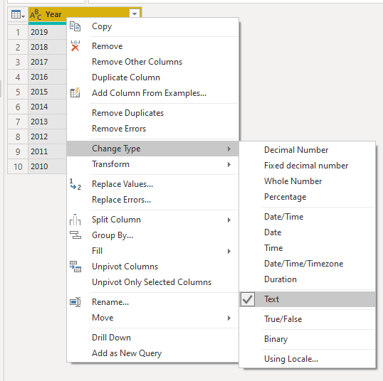
So we don’t have to do a text conversion inside the function, go ahead and change the type of column for “Year” in SeasonData to Text. Right-click the column header, select “Change Type” and select “Text.”
Load the Data
Now the fun part, calling the function and watching the data load!
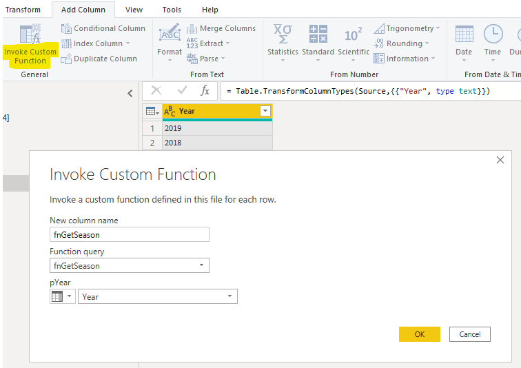
While in the SeasonData table, activate the “Add Column” tab and select “Invoke Custom Function.” For the pYear value, make sure “Column Name” is selected, and choose “Year” in the field dropdown. Click OK and a new column will be created. This will be a table column, containing a table in each cell.
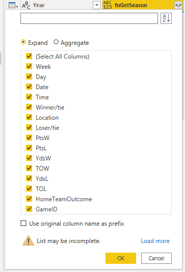
By clicking the expand contents button in the column header , we can expand all of the contents, with the Year column propagating next to the information about each game. Uncheck the “Use original column name as prefix” option and click OK.
A preview of data will be displayed in the SeasonData table. You may notice that the field types are of the “Any” category. We need to model those explicitly for the best results. The points (PtsW = winning team points, PtsL = losing team points), number of yards (YdsW, YdsL), turnovers (TOW, TOL), and GameID fields should be changed to Whole Number, with the remaining fields stored as Text.
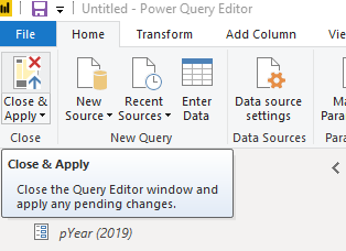
Load the data into the model by clicking “Close and Apply” from the Home Ribbon. This will load data from the last 10 seasons into the SeasonData table. It is probably a good idea to save the workbook at this point. Click the save button and save the file as “NFL Seasons.pbix.”
Create Columns and Measures
We might want to distinguish regular-season games from playoffs. To do this, remember we have a field called “Week” with week number of the regular season and the round of playoffs. Since the week number of the regular season is at most 2 digits and the playoffs are longer text values (SuperBowl, WildCard, etc.), we can use the LEN function inside an IF statement to classify the game as Regular Season or Playoffs. Right-click on the SeasonData table and select “New Column.” In the formula editor, type the following:
GameType = if(len(SeasonData[Week]) < 3, "Regular Season", "Playoffs")
It is a good practice to create explicit measures in Power BI that define the calculations we want to perform, rather than relying on aggregations of the columns as they are dropped into visuals. A simple measure is the count of the number of games, accomplished by counting the number of distinct GameID values. Right-click on SeasonData and select “New Measure.” Populate the formula bar with the following text:
Games = DISTINCTCOUNT(SeasonData[GameID])
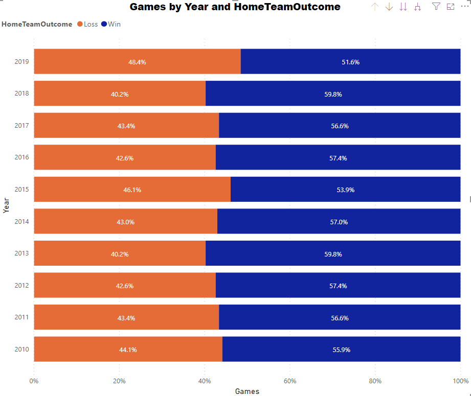
With this measure, we can create several visualizations, including counting the number of games where the home team wins/loses by year and game type (see below for a graph showing the home team wins and losses by year in the regular season since 2010). 2019 saw the lowest home team winning percentage in the last 10 years.
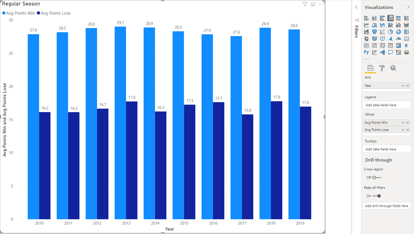
Another example can be created showing the average score in the regular season. Create the following two measures:
Avg Points Lose = AVERAGE(SeasonData[PtsL])
Avg Points Win = AVERAGE(SeasonData[PtsW])
Then, create a clustered column chart and filter the data where GameType = “Regular Season” as shown below.
Summary
With these simple measures as a guide, there are numerous types of data slices and analyses you can perform with Power BI. Some ideas include Turnover Margin Winning Team (TOL-TOW) and Winning Margin (PtsW – PtsL). Additional modeling can glean home field advantage calculations and even calculate correlations between turnover margin, yardage margins, and wins.
This post has highlighted how the web connector in Power BI, in conjunction with parameters and functions, can quickly retrieve data from the web and enable advanced visualizations and insights. A known limitation is that this type of data source (dynamic, in that Power Query cannot determine the structure until runtime) may not be refreshed reference link once it is published to the Power BI service.
 KiZAN is a Microsoft National Solutions Provider with numerous gold and silver Microsoft competencies, including gold data analytics. Our primary offices are located in Louisville, KY, and Cincinnati, OH, with additional sales offices located in Tennessee, Indiana, Michigan, Pennsylvania, Florida, North Carolina, South Carolina, and Georgia.